The files were showing as bz2 extensions until I installed winRAR and they now show as winRAR archive files in explorer and have changed extensions in the title such as .nc,.img, .xyz
Does anyone know of a file converter I could download that will let me convert them to a Gplates format?
If that doesn’t work then it might be that the “.nc” file was not extracted properly from the “.bz2” file (I’m not sure what WinRAR did, but you might need to get it to explicitly extract, if it hasn’t done so already).
Looks like you’re looking at the old 2008 data. Maria Seton has published a new set of data this year:
Seton, M., Müller, R. D., Zahirovic, S., Williams, S., Wright, N., Cannon, J., Whittaker, J., Matthews, K., McGirr, R., (2020), A global dataset of present-day oceanic crustal age and seafloor spreading parameters, Geochemistry, Geophysics, Geosystems, doi: 10.1029/2020GC009214
Thanks, I’m brand new to the program. The data that Sabin linked me to is already in the .nc format. I’m looking for a data set that shows or will enable me to find global spreading rates (mm/yr) at mid ocean ridge locations over a particular time period, the longer the geological time period the better. Would this data show that?
I followed the tutorial 3.1 and have imported all of the .nc spreading rate files as rasters. I wasn’t prompted to enter any geo-referencing coordinates, however, as the guide shows. All that has happened is parts of the globe have became coloured. There’s no indication of what to do next and I’m quite lost.
Since this data set contains present-day grids, each pixel in the spreading rate grid came from a mid-ocean ridge at the age of the same pixel in the associated age grid. (I’m not sure if that answers your question.) And the age grid shows that some pixels are further back in time than others…
More recent versions of GPlates read the georeferencing data embedded in the raster file, and only prompt you to enter it if the file does not contain it.
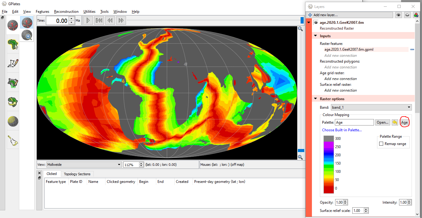
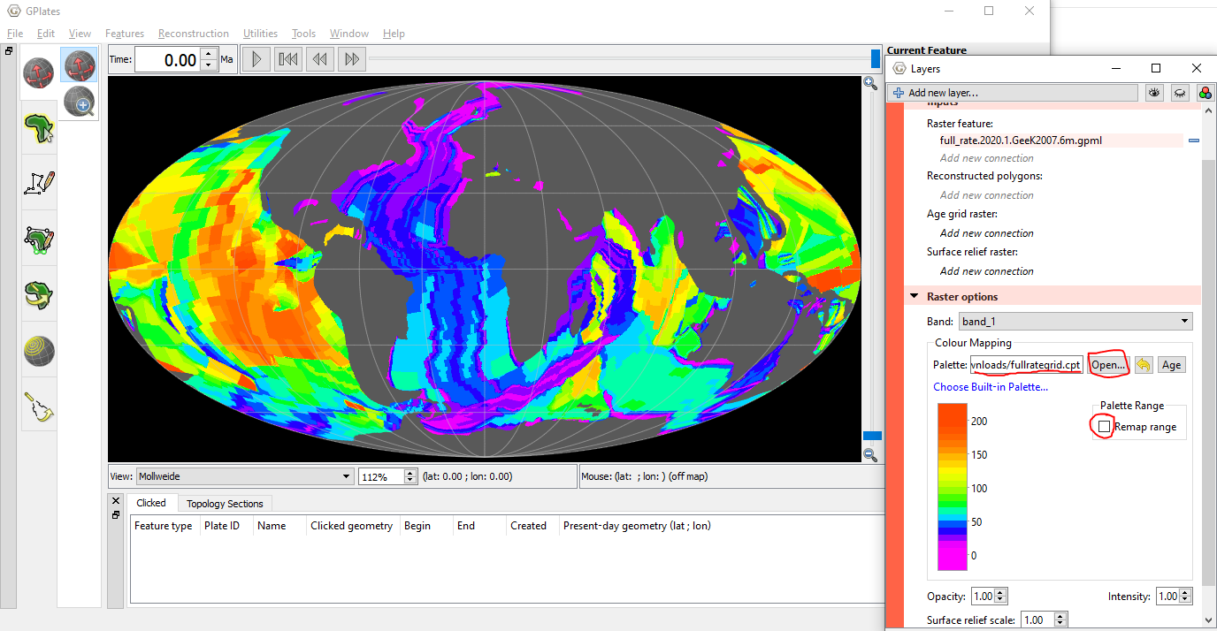
Firstly, you can expand the raster layer to see the colour palette that maps the spreading rate values (mm/yr) to colours…
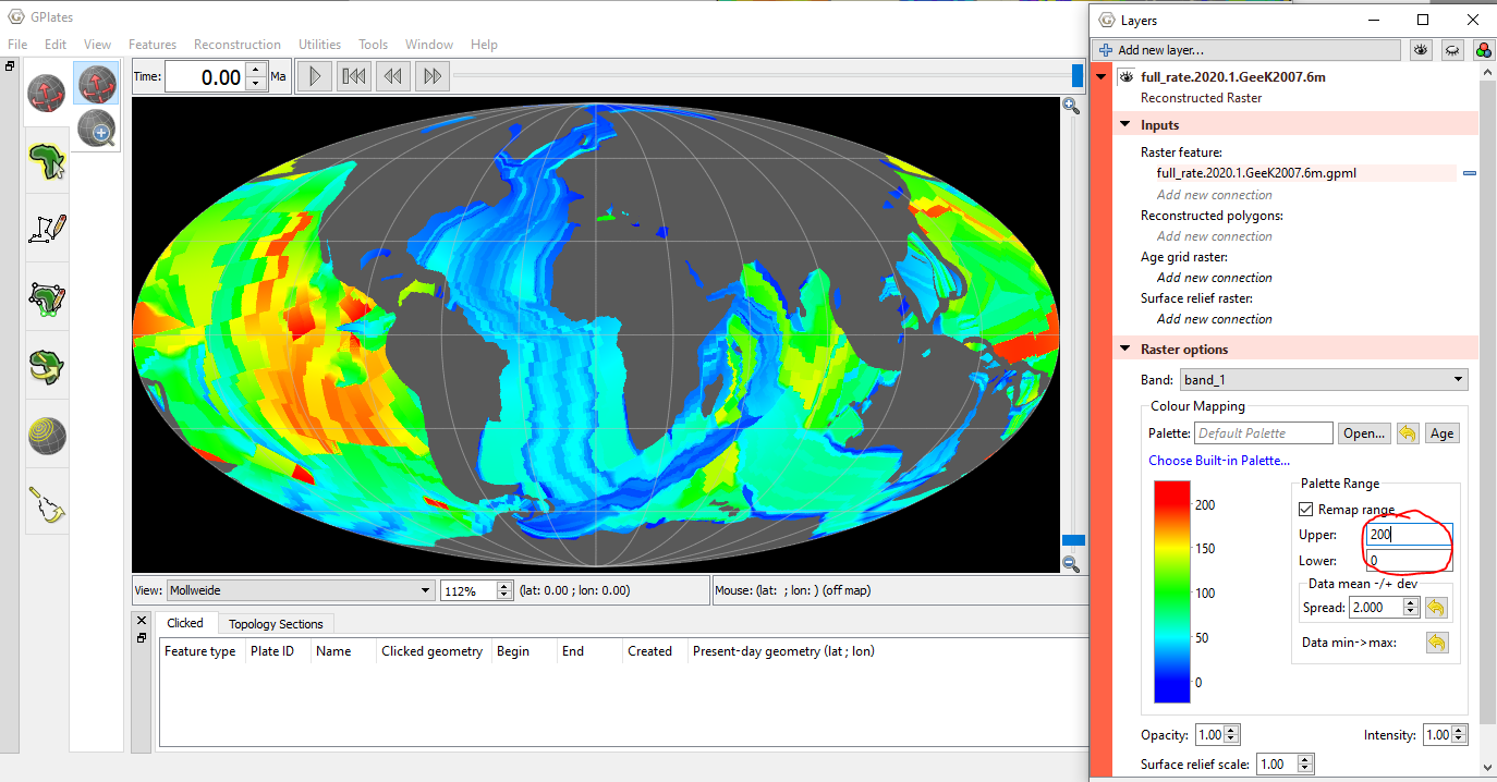
Then you can then modify the palette range (eg, by clicking Data min->max) or manually entering lower/upper values for the range. Here I’ve changed the range to [0, 200]…
Note that I’ve un-ticked the Remap range check box so that the natural range of the CPT is used instead. Here’s a copy of the contents of that CPT file where you can see that the range covers [0, 200] (each line is lower_spreading_rate lower_RGB_colour upper_spreading_rate upper_RGB_colour)…
Thanks for the reply. I’ve yet to follow the steps you’ve described because there was an error (19153) reading the source raster file cache for the .NC file when I tried importing. A rebuild was attempted and then the notice ‘Fileformatnotsupportedexception: detected a partially written source raster file cache’
Is there a certain order that the files from the age grid folder need to be added in? Most of them loaded fine. It was just the 6 larger age raster files that caused the program to freeze, not respond and the error message to show. I need them all imported.
Update I tried downloading the files again but I’m having the same problem. Gplates crashes when I try to import the age based rasters from the Seton et Al 2020 dataset linked by Sabin.
There is also a slight discrepancy in the file sizes. For example on my computer the GTS2012.1m NC file is 21.606 MB and on the website it states 206 M (which I assume is MB). There are slight differences for the others too.
Am I right in assuming that most spreading rates don’t change for thousands if not hundreds of thousands of years? Is that still true for mid ocean ridges?
I’m looking for spreading rates for each mid ocean ridge around the globe, so that will be about 20. If the rate has changed at a ridge location and the data set shows this then I’ll gather all of them, but I need some guidance on how to do this.
I’m new to the gplates program and confused as to why there are so many age and spreading rate files in the dataset? How would I know which ones to use to obtain this information? Do certain files need to be imported and viewed together in gplates to obtain this?
A few of the larger age files are causing the program to freeze and not respond when I try to import them as normal and time dependent rasters. I tried downloading them again but this didn’t resolve the issue.
Do you think this is the right dataset to look at for what I need?
You can add them in any order. I’m assuming you’re importing each raster separately (not as a time-dependent import).
It might be that the files are only downloading partially for some reason. You can also try importing them in other software that loads NC (such as GMT). But yeah, I would make sure the downloaded file sizes match first.
The larger ones take longer to import. GPlates appears to hang but it’s just processing - perhaps try waiting a little longer - for example the 206MB GTS2012.1m NC takes me 8 minutes to import (and writes 1.5GB worth of data into two new .cache files for faster loading next time - this will all be improved in the long term, both for disk usage and import speed). By the way, that’s quite high resolution (1m = 1 minute = 1/60 degree resolution) - perhaps start out with 6 minute resolution (.6m) which will import much faster (almost instantly).
That’s a pretty small time scale and the rotations in the rotation file (used to calculate the spreading rates) are at times on the order of millions of years, so I’m not sure what can be said at smaller time intervals. So I’m not really sure.
Have a look at the Readme file in the same directory as the grids. It covers what each individual file is. Also the associated paper might help.
Do these datasets cover rates at mid ocean ridges? If I were to locate each one using a specific latitude and longitude, or would I need to take extra steps to cover the mid ocean ridges? I notice there is a tutorial dealing specifically with them.
So the natural range of the CPT files, corresponding to a chosen palette colour scheme with various shades between the intervals of 50 mm/yr will enable me to find the exact spreading rate values at each ridge location? What exactly do lower and upper spreading rate indicate? Is it just the size of the value?
It sounds as if the spreading rates are within the CPT files. There are a few in the dataset, but the correct one is ‘fullrategrid’? I’m aiming for a palette like the one in your second to last screen shot, where it is broken into many shades.
How did you load the contents of the palette to show the full range and the individual values? Is it detailed which shade each individual value corresponds to? This is where I’m getting confused.
I only want spreading rates from the most recent geological period, if the datasets go back millions of years, so for what I need should I just load the most recent age raster file, with the fullspreading rate file? This is where I’m confused again, I don’t know which ones they are out of the Seton et al data. I’ve read the readme and I’m still wondering what the z value is? Is it part of the file name?
If someone could tell me what age file the youngest is and which one(s) to upload out of the NC, cache, GRD and gpml files that would be a huge help. I’d need the same info for the spreading rate files. Is it full_rate.2020 or full_rate_bands.2020?
I should be fine once I know these answers. Thanks very much.
If you are looking at present-day mid-ocean ridges, then yes. The grids are only at present day, so they don’t show the positions of those same present-day ridges reconstructed to their positions at past times. So yes, you can take a lat/lon position somewhere along a mid-ocean ridge (in its present-day position) and look it up in the spreading rate raster.
The tutorial is more about creating mid-ocean ridge features that existed at past times.
I don’t know about exact, but you can position your mouse at your specific latitude and longitude on the globe and see what colour is under the cursor and then visually look up that colour in the colour palette table and see roughly what numerical value it has (eg, is it slow, fast, etc).
The CPT file I used in my screenshot (fullrategrid.cpt) has lower/upper bounds of 0/200. These take raster values between 0 and 200 and assign them colours. And the raster values are in units of mm/yr (because that’s what it says in the README file in the same directory as the raster files). So that means the range of colours, shown in the palette, is for values between 0 and 200 mm/yr (with raster values below 0 mm/yr and above 200 mm/yr clamped to those 0 and 200 mm/yr colours respectively).
Well, the spreading rates are values in the raster, so you can’t really change them (unless you somehow modify the raster), but you can change the range of values displayed in GPlates (and what colours that range is mapped to) using the various approaches I covered in a previous post. And yes, I used the fullrategrid CPT with the full_rate... rasters.
I clicked the open button - the button circled in red in the screenshot showing usage of that CPT file - and then located the CPT file in the file system. Once it’s loaded (and I’ve un-checked remap range as I mentioned above) then the CPT file takes over (ie, the range and colours are completely determined by the CPT file) with the raster simply providing the input z values to be mapped to colours.
It’s detailed in the CPT file (as I showed in a previous post - perhaps just open the CPT with your favourite text editor), and you can see some values in the colour palette shown in GPlates.
It’s a present day age raster - it shows the age of oceanic crust at present day. You can load that, and load the spreading rate raster (also at present day).
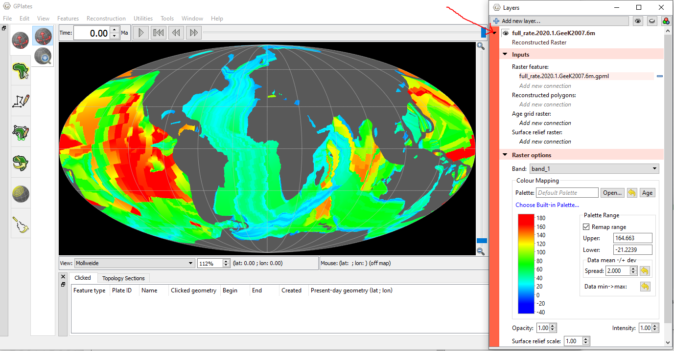
The spreading rate raster I loaded has the following description in the README file…
full_rate.2020.1.GeeK2007.6m.nc		NetCDF-4 formatted file (compatible with GMT5 and above)
                                    The geographic grid spans longitudes from -180 to
                                    +180 and latitudes from 90 N to -90 N.
                                    Z value is the full spreading rate (mm/yr).
                                    6 minute resolution, gridline-registered.
                                    Timescale used is Geek and Kent (2007).
…so the z value is the full spreading rate in units of mm/yr as noted above (the filename also contains full_rate).
Try importing age.2020.1.GeeK2007.2m.nc and full_rate.2020.1.GeeK2007.6m.nc. Once you’ve imported them you’ll get associated GPML files. The next time you open GPlates you can just open the GPML files (instead of having to import the rasters again) using File > Open Feature Collection. Don’t worry about the cache files.
I’m still a bit confused with the fullrategrid.CPT file. Reading it in my text viewer I can see that there are 36 values. I assume that each shade of the colour palette covers each value, in ascending order? When I opened it in a text viewer they weren’t in order but I assume they have to be? 255 is the highest value and so before I unticked remap range I set that as the upper value and 0 as the lower, is that right?
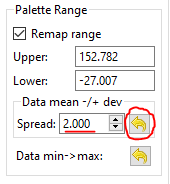
I’m also confused what the spread value does? Its 2.000 by default but the palette looks more ordered with 1.000.
I’m not going to touch the opacity and intensity or surface relief.
Is there a way to expand the palette so that I can see the shades clearer or larger? I’m finding them hard to discern because the palette is so small and cramped
I’m not quite sure which 36 values you mean. But in the following (fullrategrid.cpt) there are 20 colour slices (the first 20 rows) which define colours in the z (ie, raster value) range from 0-200, and 3 colours B, F and N at the end which define colours outside that 0-200 range (B is background colour for z < 0, F for foreground z > 200 and N for undefined, or NaN, values) - have a look at the GMT makecpt command.
…so the first line (colour slice) says values between 0 and 10 are assigned the Red Green Blue colour 255 0 255 …
0 255 0 255 10 255 0 255
…and the 255 is part of the colour (as opposed to the z raster value) that, since the colour values are 8-bit, represents the maximum intensity of the colour component (whether that’s red or green or blue). So 255 0 255 is full red, no green, full blue.
And I don’t think the z slices have to be ordered by value.
The spread value is just a convenient way to define the minimum and maximum z value that you are remapping. When you are remapping you are essentially taking the z values in the CPT file (in the above case 0 to 200) and remapping them to a new min/max range of your choosing. You can either explicitly choose that min/max range (by manually entering Lower and Upper) or you can enter a Spread value and then click the button in the following screenshot to get GPlates to set the Lower and Upper values based on the mean and standard deviation of all the values in the raster being displayed…
…and in our CPT example above (with z range 0-200) this means Lower gets remapped to 0 and Upper gets remapped to 200 when looking up the colours in the CPT file. This means any raster value less than Lower gets clamped to the background B colour, and any raster value greater than Upper gets clamped to the foreground F colour, with raster values in between getting the regular colours.
The default is 2.0 because that better suits most rasters in general because it covers a larger range of the raster values, but you can set it to any value (and the project file will remember it).
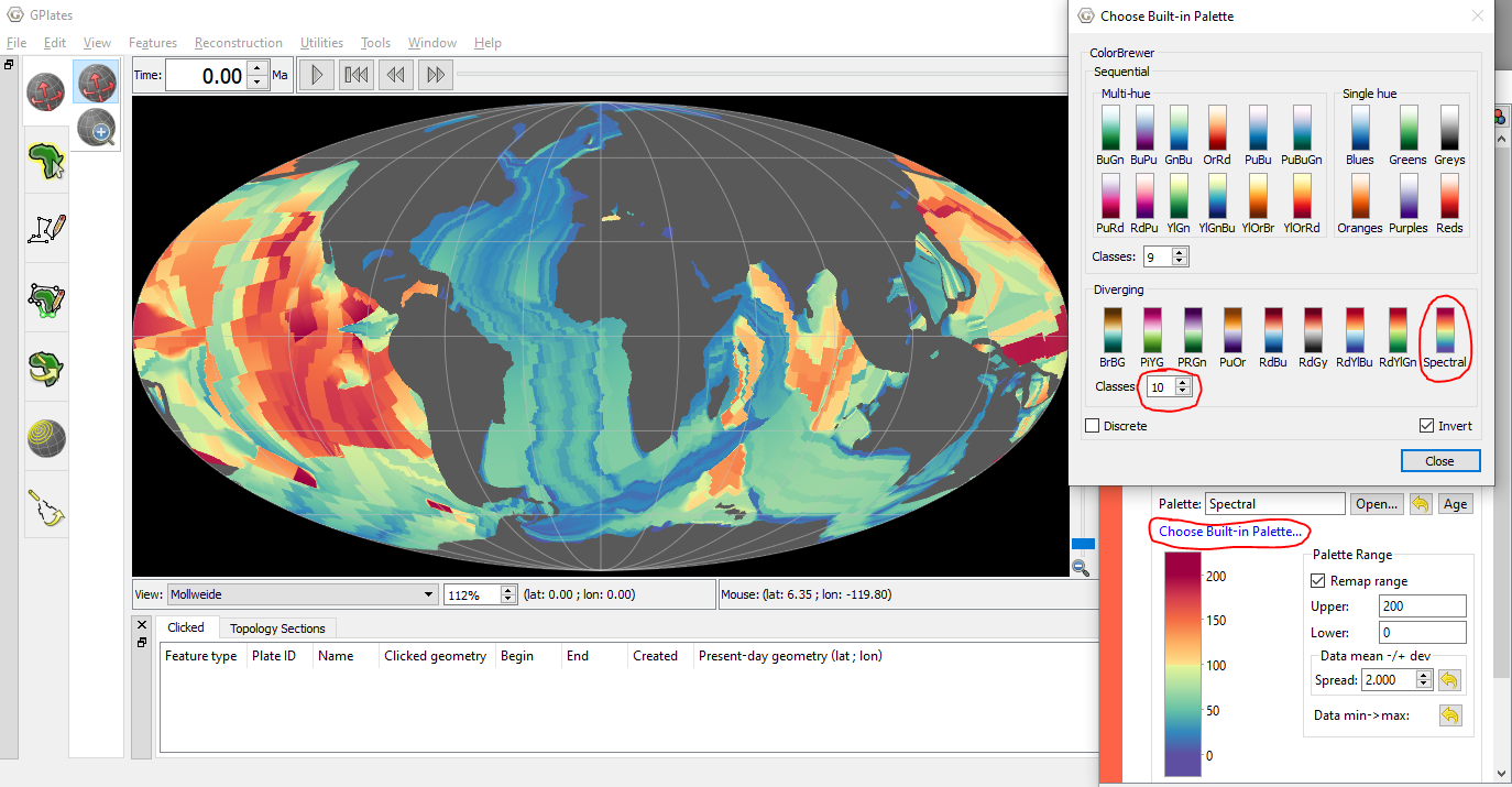
You can remap the z range and change the min/max values, but that might not achieve what you want, in which case you may want to modify/add more colour slices in the CPT file so that the 0-200 range will see more colour variation. Alternatively try an inbuilt colour palette or try loading a different CPT file - the GMT site lists its palettes here and also links to additional external colour tables (eg, cpt-city).
Would you be able to tell me the simplest way to find which shade (or ‘colour slice’) corresponds to which particular mm/yr value? Am I right in assuming that one colour slice corresponds to one value in the .cpt file? It sounds like more than one colour may correspond.
This is based on the age.2020.1Geek2007.2m.nc and full_rate.2020.1.Geek2007.6m.nc rasters which I’ve imported.
I’d like to be able to read the .cpt contents so that I can simply assign a mm/yr value to each colour slice in the raster palette, starting from the bottom of the palette going upwards to the top. Once I know this I can just look at the colour slice of the lat/long area I’m studying and know it’s value in mm/yr.
This is all I’m looking for. For someone brand new to the program I’d like to keep things as simple as possible.
Depends what you mean by “value”. If you mean z (raster) value then no, it corresponds to a range of z values. For example, the colour slice 0 255 0 255 10 255 0 255 corresponds to the range of z values 0 to 10.
You might be getting confused by the fact that one row (slice) of the CPT file contains two colours…
z_lower RGB_lower z_upper RGB_upper
…where if z_lower < z < z_upper (in other words a particular raster z value falls within that slice) then the colour assigned to z is linearly interpolated between RGB_lower and RGB_upper. But in the particular CPT file we’re looking at, the lower and upper RGB values in each slice are the same (RGB_lower = RGB_upper), and so any z value within a particular slice will be assigned the same colour.
…and so if you see the colour 1st_z_RGB on the globe (at a particular lat/lon) then you know the spreading rate is between 0 and 10 mm/yr. Which brings us back to why the original fullrategrid.cpt CPT file is structured this way.
There are more than 20 colour slices in the palette, and the markings aren’t lined up to mark every 5 slices, so I’m not sure how to read it. I.e. 50 and 100 aren’t resting on one particular slice. Why isn’t 0 at the very beginning? What values would correspond to the slices beneath 0?
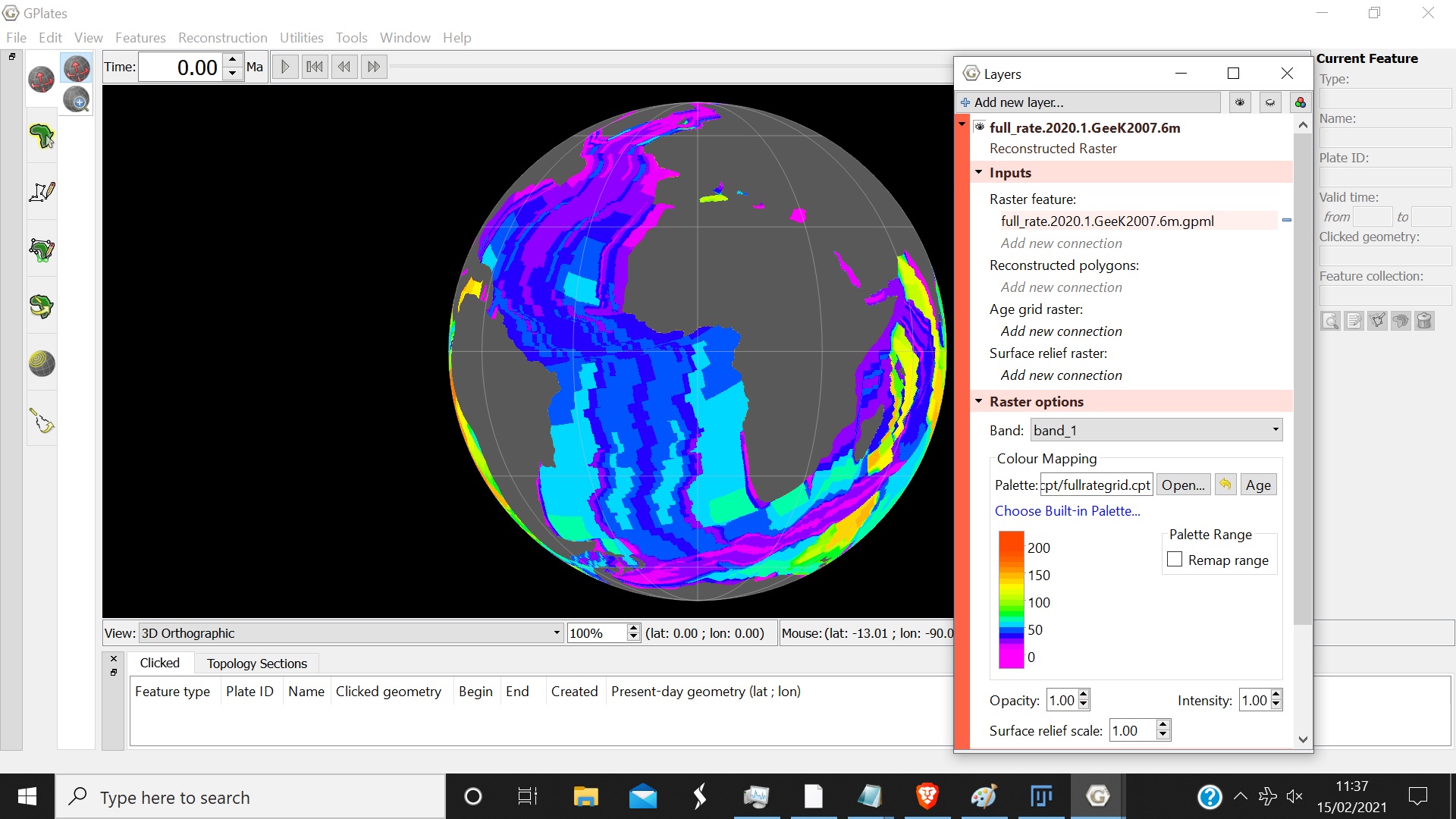
Also, as you can see, in the screenshot, after unticking ‘remap range’ the palette shrinks significantly. I’m finding it really difficult to actually see the individual slices with it being that small. I can make out some of the slices, but the ones at the top and bottom appear to blend together - making it hard to see the individual slices.
So the z value is just the incremental number, i.e. if the colour slice values increase by 10 mm/yr then the z value is 10? Does that mean that values falling in between the increments of 10, i.e. 126 mm/yr, would be assigned their own colour slice in between the increments?
Let me know if the screen shots that I’ve attached look correct.
Thanks
So that it can show the colour below 0 (the background B colour).
The background B colour is for all z values lower than zero.
I would suggest to go through the thread again and try to understand the CPT format as I’ve described it. And if that’s insufficient then look at the following GMT description of regular CPTs (since CPT is a GMT format).
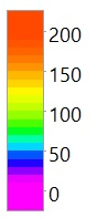
The spacing of the marks is independent of the CPT file (ie, they are not necessarily lined up with the colour slices in the CPT). They’re just spaced enough to not be too crowded and not too sparse…
…so it’s just meant to give you an idea of the values. If you have 20 colour slices then you’re not going to be able to read exact values for each colour. In which case perhaps you can start with this tutorial on the GMT site to try to display the colour bar in higher resolution (and perhaps with more markings but I’m not very familiar with GMT plotting).
As I mentioned I think it’s best if you review this thread and look at the GMT site. Good luck